
Knowledge Centre
Sharing the expertise behind successful engineering projects.
Airflow Simulation: From Flow Fields to Engineering Decisions
Airflow problems rarely begin with a lack of airflow.
More often, the problem is where the air goes, how much pressure is lost along the way, and whether the flow reaches the parts of a system that actually need it.
A fan may be capable of delivering the required flow rate. A ventilation system may appear adequately sized. An enclosure may have sufficiently large openings. Yet once the system is assembled, some regions can remain poorly ventilated, components can run hotter than expected, or pressure losses can become significantly higher than anticipated.
This is where computational fluid dynamics, or CFD, becomes useful.
The value of airflow simulation is not in producing colourful velocity contours or attractive streamlines. Its real value is in understanding the physical behaviour of a system before hardware is built, identifying the mechanisms responsible for poor performance, and giving engineers a quantitative basis for changing the design.
Airflow Is a Distribution Problem
Consider a system with a single air inlet and several possible flow paths.
The total airflow entering the system may be exactly what was expected. That does not mean the airflow is distributed correctly.
Air responds to pressure gradients and preferentially moves through paths with lower resistance. A relatively small change in geometry can therefore alter the distribution substantially.
This becomes important in many engineering systems, including:
- electronics enclosures
- cooling ducts
- manifolds
- ventilation systems
- heat exchangers
- battery cooling systems
- industrial equipment
- machinery enclosures
- HVAC systems
- automotive components
The engineering question is therefore rarely just:
How much air is moving through the system?
It is more often:
Where is the air moving, what is driving that behaviour, and is the resulting flow sufficient for the design objective?
That distinction is fundamental to effective airflow analysis.
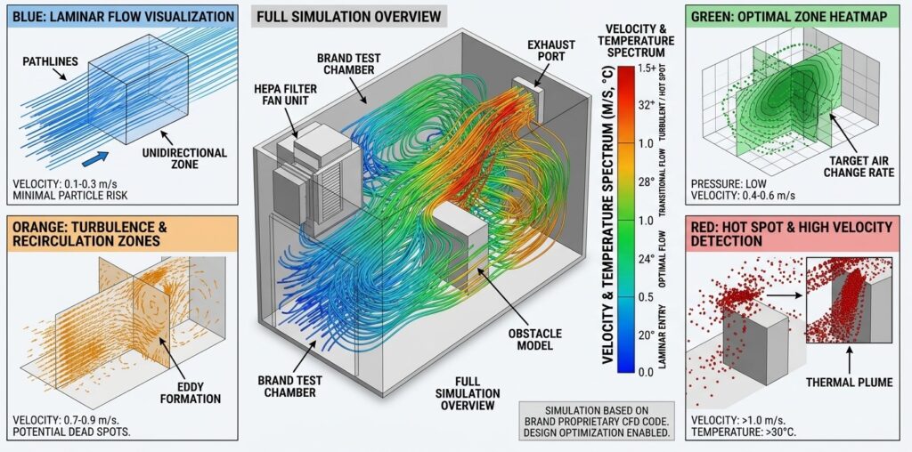
The Physics Behind the Flow
At its foundation, an airflow simulation solves equations describing conservation of mass, momentum and, where required, energy.
For an incompressible fluid, conservation of mass is expressed as:
∇ · u = 0
where:
- u is the velocity vector
- ∇ · u represents the divergence of the velocity field
The momentum equations describe how the velocity field changes as a result of pressure gradients, viscous effects and other forces.
When temperature is important, the energy equation must also be considered. This introduces coupling between airflow and thermal behaviour.
The equations themselves are well established. The engineering challenge is deciding which physical effects matter for the particular system and how they should be represented.
Reynolds number and flow behaviour
The Reynolds number provides an indication of the relative importance of inertial and viscous effects:
Re = ρUL / μ
where:
- ρ = fluid density
- U = characteristic velocity
- L = characteristic length
- μ = dynamic viscosity
The Reynolds number helps indicate whether laminar, transitional or turbulent behaviour is likely to dominate.
This matters because turbulence influences:
- mixing
- pressure loss
- wall shear
- flow separation
- heat transfer
- flow distribution
However, Reynolds number does not determine the complete behaviour of a system by itself. Geometry, surface conditions, pressure gradients and thermal effects can all change the resulting flow.
Flow Separation Can Change the Design Completely
One of the most important phenomena in practical airflow systems is flow separation.
Air does not necessarily follow a surface simply because the geometry initially appears smooth. Under an adverse pressure gradient, the boundary layer can lose momentum and separate from the wall.
The result may include:
- recirculation
- increased drag
- higher pressure loss
- local turbulence
- reduced effective flow area
- uneven cooling
- unexpected vibration or noise
A duct transition that looks acceptable in a CAD model can therefore produce very different behaviour once air is flowing through it.
This is one reason why geometry optimisation based only on dimensions or static calculations can be misleading.
Geometry Is Part of the Physics
In airflow analysis, geometry is not simply the environment surrounding the fluid.
It determines the available flow paths, the pressure losses and the locations where the flow accelerates, separates or recirculates.
Consider an electronics enclosure.
Changing the position of a ventilation opening by a relatively small distance can alter the entire internal flow pattern. Air may bypass a heat-generating component and move directly towards the outlet. Alternatively, the same change may create a more direct flow path and improve cooling.
The total airflow may remain almost unchanged.
The temperature distribution may not. That is why CFD is particularly useful when the design objective depends on flow distribution rather than total flow rate
Boundary Conditions Matter More Than Many People Expect
A CFD model can contain millions of computational cells and still produce a poor engineering result if the physical boundary conditions are wrong.
Depending on the system, the engineer may need to define:
- inlet mass flow
- inlet velocity
- inlet pressure
- outlet pressure
- fan performance
- wall conditions
- heat generation
- ambient temperature
- porous resistance
- rotating components
- thermal properties
Choosing between these approaches requires an understanding of the actual physical system.
For example, specifying a fixed airflow rate at a fan inlet may be appropriate for one analysis but physically inappropriate for another. If the purpose is to determine the operating point of a fan installed in a real system, the interaction between fan performance and system resistance becomes important.
The distinction is significant.
A model can be mathematically stable while still representing a physical condition that would never occur in the real system.
Fan Capacity Is Not the Same as System Airflow
Fan specifications are often misunderstood during early design.
A fan may be advertised with a maximum airflow under near-zero static pressure. Once the fan is connected to a real system, the actual flow rate depends on the resistance of that system.
Filters, ducts, grilles, heat exchangers, bends, contractions, expansions and other restrictions all contribute to pressure loss.
The operating point occurs where the fan performance and system resistance are compatible.
This relationship can be expressed as:
ΔP_fan(Q) = ΔP_system(Q)
where:
- ΔP = pressure difference
- Q = volumetric flow rate
A typical system resistance relationship can often be approximated as:
ΔP_system ∝ Q²
or, more explicitly:
ΔP_system = KQ²
where K represents the effective resistance of the system.
This is why analysing the fan separately from the system can produce an unrealistic expectation of actual airflow.
The useful engineering question is not:
What is the maximum airflow of the fan?
It is:
What flow rate will the complete system actually operate at?
Thermal Management Is Often an Airflow Problem
Airflow and thermal analysis are frequently inseparable.
Consider an enclosure containing several electronic components with different heat loads.
The cooling problem can be viewed as a coupled process:
Heat generation → temperature rise → density change → air movement → heat removal
With forced convection, the fan strongly influences the flow field. With natural convection, buoyancy can become the driving mechanism.
In many practical systems, both effects exist at the same time.
This is known as mixed convection.
A system can therefore behave very differently under different operating conditions. A design that performs adequately at low ambient temperature may have considerably less thermal margin at elevated ambient temperature.
This is why a temperature contour by itself is not enough.
The engineer needs to understand why the temperature distribution exists.
An Engineering Example: Cooling an Electronics Enclosure
Consider an enclosure containing three heat-generating components, with a fan mounted near one side and ventilation openings on the opposite side.
Assume:
- enclosure dimensions: 400 mm × 300 mm × 150 mm
- ambient temperature: 25 °C
- total internal heat generation: 120 W
- one axial fan
- defined inlet and outlet openings
A simple engineering assumption might be that the fan will distribute air reasonably evenly across the enclosure.
CFD can test that assumption.
The first analysis might reveal a dominant flow path between the fan and outlet, with relatively little air reaching one of the heat-generating components.
The velocity field may show a high-speed region near the outlet and a low-velocity region around the poorly cooled component.
The temperature field may then show a corresponding local thermal hotspot.
At this point, the simulation has answered a much more useful question than simply reporting average airflow.
It has identified the mechanism responsible for the thermal problem.
The geometry can then be modified.
Possible changes might include:
- relocating the inlet
- increasing the outlet area
- adding a flow guide
- modifying internal obstructions
- changing component placement
- introducing additional ventilation
The modified geometry can be simulated again and compared against the original configuration.
This creates a useful engineering loop:
Design → Analyse → Identify → Modify → Re-analyse
The objective is not to generate a better-looking CFD plot.
The objective is to produce a better-performing design.
Flow Distribution in Manifolds
A similar problem occurs in manifolds where one inlet supplies several branches.
Suppose four outlets are geometrically similar and the total required flow is known.
It is tempting to assume that each outlet will receive approximately one quarter of the total flow.
That assumption may not hold.
Pressure losses through the branches and the geometry of the manifold can create significant differences in flow rate.
A CFD model can determine the flow through each branch and identify where the imbalance originates.
For example, a first-pass design might produce:
- Outlet 1: 35% of total flow
- Outlet 2: 28%
- Outlet 3: 22%
- Outlet 4: 15%
The total flow is correct, but the distribution is poor.
A geometry modification can then be introduced to increase resistance in the dominant branch or reduce resistance in the weaker branches.
The objective is not necessarily to minimise pressure loss everywhere.
It may instead be to achieve the required flow uniformity.
That is an important distinction in engineering optimisation.
Mesh Quality and Why More Cells Are Not Always Better
The computational domain must be divided into a mesh before the governing equations can be solved numerically.
Mesh resolution affects the ability of the model to capture important physical features.
Areas that may require additional resolution include:
- boundary layers
- narrow passages
- sharp geometric changes
- wakes
- separated flow
- regions with strong temperature gradients
However, increasing mesh size indefinitely is not a substitute for good modelling.
The important question is whether the predicted engineering quantity has become sufficiently insensitive to further mesh refinement.
For example, a mesh study might produce:
| Mesh | Cells | Predicted pressure drop |
| Coarse | 0.8 million | 91 Pa |
| Medium | 1.7 million | 87 Pa |
| Fine | 3.5 million | 86 Pa |
| Very fine | 6.8 million | 85.7 Pa |
The useful information is not that the last mesh contains the most cells.
The useful information is that the predicted pressure drop is becoming relatively insensitive to further refinement.
For the pressure-drop quantity of interest, the change from the fine mesh to the very fine mesh is only:
(86.0 − 85.7) / 86.0 × 100 ≈ 0.35%
That provides evidence that further refinement is having a relatively small effect on the selected engineering result.
Mesh independence does not mean that every aspect of the flow is perfectly resolved. It means that the chosen quantity of interest has become sufficiently stable for the purpose of the analysis.
Turbulence Modelling Requires Engineering Judgement
Most practical engineering flows are turbulent or contain regions of transitional behaviour.
Resolving every turbulent scale directly is generally computationally impractical for industrial design problems. Instead, turbulence models are used to represent the effects of unresolved turbulent motion.
Common approaches include:
- Reynolds-averaged Navier–Stokes, or RANS
- k–ε models
- k–ω models
- SST formulations
- transitional models
- Large Eddy Simulation, or LES
There is no universally correct turbulence model.
The appropriate approach depends on the physics being investigated, the geometry, the expected flow regime and the required level of fidelity.
For many industrial applications, RANS-based methods provide a practical balance between computational cost and predictive capability.
For highly unsteady flows, strong separation or other complex phenomena, a more advanced modelling approach may be justified.
The important point is that model selection should follow the engineering problem, not the other way around.
A Converged Solution Is Not Automatically a Correct Solution
This distinction is essential.
A CFD solver can reach convergence while the model still contains unrealistic assumptions.
There are three different questions:
Has the numerical solution converged?
The calculated quantities and residuals have stabilised sufficiently.
Has the numerical problem been solved correctly?
The discretisation, mesh and numerical method behave as intended.
Does the model represent the physical system adequately?
The model predictions agree sufficiently with physical behaviour for the intended purpose.
The last question is validation.
Where suitable experimental information is available, CFD results should be compared with measurements such as:
- pressure
- temperature
- flow rate
- velocity
- system performance
The purpose is not to make the simulation “look right”.
It is to establish confidence in its ability to predict the behaviour that matters.
This distinction between verification and validation is important because numerical convergence alone cannot demonstrate physical accuracy.
Understanding the Results
A CFD project can generate a large amount of data.
Not all of it is equally useful.
Velocity
Velocity contours can identify acceleration, low-flow regions and potential flow restrictions.
But the important engineering question is why the velocity is high or low and whether that behaviour affects system performance.
Pressure
Pressure distribution can reveal where energy is being lost and help identify inefficient geometry.
Streamlines
Streamlines are particularly useful for understanding dominant flow paths, recirculation and bypass flow.
They should, however, be interpreted correctly. A streamline is a visual representation of the calculated velocity field, not a physical photograph of individual air particles.
Temperature
Temperature distributions show whether heat is being removed effectively and where thermal margins may be reduced.
Pressure drop
Pressure drop is often a key system-level metric because it directly influences required fan performance.
A useful simulation therefore focuses on the quantities that matter to the engineering decision rather than generating every possible contour available in the solver.
Sensitivity Analysis: Which Assumptions Actually Matter?
A single simulation represents one combination of inputs.
Real products do not operate at one perfectly fixed condition.
Ambient temperature changes. Fan speed changes. Heat generation changes. Manufacturing tolerances alter geometry. Filters become less permeable. Operating conditions vary.
Sensitivity analysis helps determine which parameters have the greatest effect on performance.
For an electronics cooling system, for example, the engineer might investigate changes in:
- fan flow rate
- ambient temperature
- component heat generation
- vent size
- vent location
- internal obstruction
- component placement
Suppose the maximum component temperature changes as follows:
| Parameter | Lower condition | Baseline | Higher condition |
| Fan flow rate | 80% | 100% | 120% |
| Maximum component temperature | 78 °C | 68 °C | 62 °C |
This simple comparison suggests that fan flow rate has a material influence on thermal performance.
A different parameter may have very little influence.
The objective is not simply to produce more simulations.
It is to identify which variables actually control the system.
That information can influence design margins, component specifications and operating limits.
Airflow Simulation Is Not a Replacement for Testing
Simulation and physical testing serve different purposes.
Testing tells us what a physical system does under specific conditions.
Simulation helps us understand why it behaves that way and allows alternative designs to be investigated without physically manufacturing every variation.
A strong engineering development process can therefore look like:
Concept → Simulation → Design optimisation → Prototype → Test → Correlation → Refinement
Where suitable test data are available, the simulation can be compared against reality.
For example, measured pressure loss might be compared with the CFD prediction:
CFD prediction: 86 Pa
Measured value: 89 Pa
The relative difference would be:
(89 − 86) / 89 × 100 ≈ 3.4%
The significance of that difference depends on the application, the measurement uncertainty and the intended use of the model.
The purpose of validation is therefore not to chase an arbitrary percentage difference. It is to understand whether the model is sufficiently predictive for the engineering decision being made.
When CFD Adds the Most Value
Airflow simulation is particularly valuable when:
- internal flow paths are difficult to visualise
- multiple competing flow paths exist
- thermal performance depends on local airflow
- pressure loss affects component selection
- geometry is complex
- experimental testing is expensive
- several design options need to be compared
- operating conditions vary
- the cost of finding a design problem late in development is high
It is less useful to perform an elaborate simulation simply because the software can do it.
The model should be proportionate to the engineering question.
A simple problem should not automatically become a million-cell CFD project.
Conversely, a complex three-dimensional flow problem should not be reduced to a single hand calculation merely because it is quicker.
From CFD Results to Engineering Decisions
The most valuable output of an airflow simulation is usually not the simulation file.
It is the decision that follows from it.
A useful CFD study might conclude that:
- an outlet is undersized
- a component is located in a recirculation region
- a fan is operating away from its intended point
- a manifold produces uneven distribution
- a pressure loss is concentrated in an avoidable restriction
- natural convection is insufficient at the required ambient temperature
- a small geometry change can significantly improve cooling
These are engineering conclusions.
They provide a direct link between computational analysis and product design.
How Twelvium Approaches Airflow Simulation
At Twelvium, airflow simulation is approached as an engineering problem rather than simply a CFD exercise.
The process begins with the question the design needs to answer.
From there, the relevant physics, boundary conditions, geometry and modelling approach are established. The computational model is then developed with appropriate mesh resolution and numerical methods, followed by verification of the solution and analysis of the quantities that matter to the design.
Where appropriate, sensitivity studies can be used to understand the effect of operating conditions and design variables.
The final objective is straightforward:
turn airflow behaviour into useful engineering information that can improve the design.
That may mean reducing pressure loss, improving cooling, increasing flow uniformity, selecting an appropriate fan, changing geometry or identifying a design limitation before it becomes a physical prototype problem.
Conclusion
Airflow simulation is most valuable when it answers a question that is difficult, expensive or uncertain to answer through intuition alone.
The engineering challenge is not simply to calculate velocity or temperature. It is to understand the physical mechanisms behind the result and determine what they mean for the design.
A credible CFD analysis therefore depends on more than a powerful solver.
It depends on the correct physical assumptions, appropriate boundary conditions, suitable turbulence and numerical models, adequate mesh resolution, verification, and where required, comparison against physical measurements.
When these elements are brought together, CFD becomes much more than a visualisation tool.
It becomes a method for reducing uncertainty, testing design decisions and understanding how a product or system will behave before the final hardware is built.